Udacity-CarND UKF 学习笔记
Udacity 自动驾驶工程师纳米学位 第二学期 无迹卡尔曼(UKF)学习笔记
项目代码GitHub链接
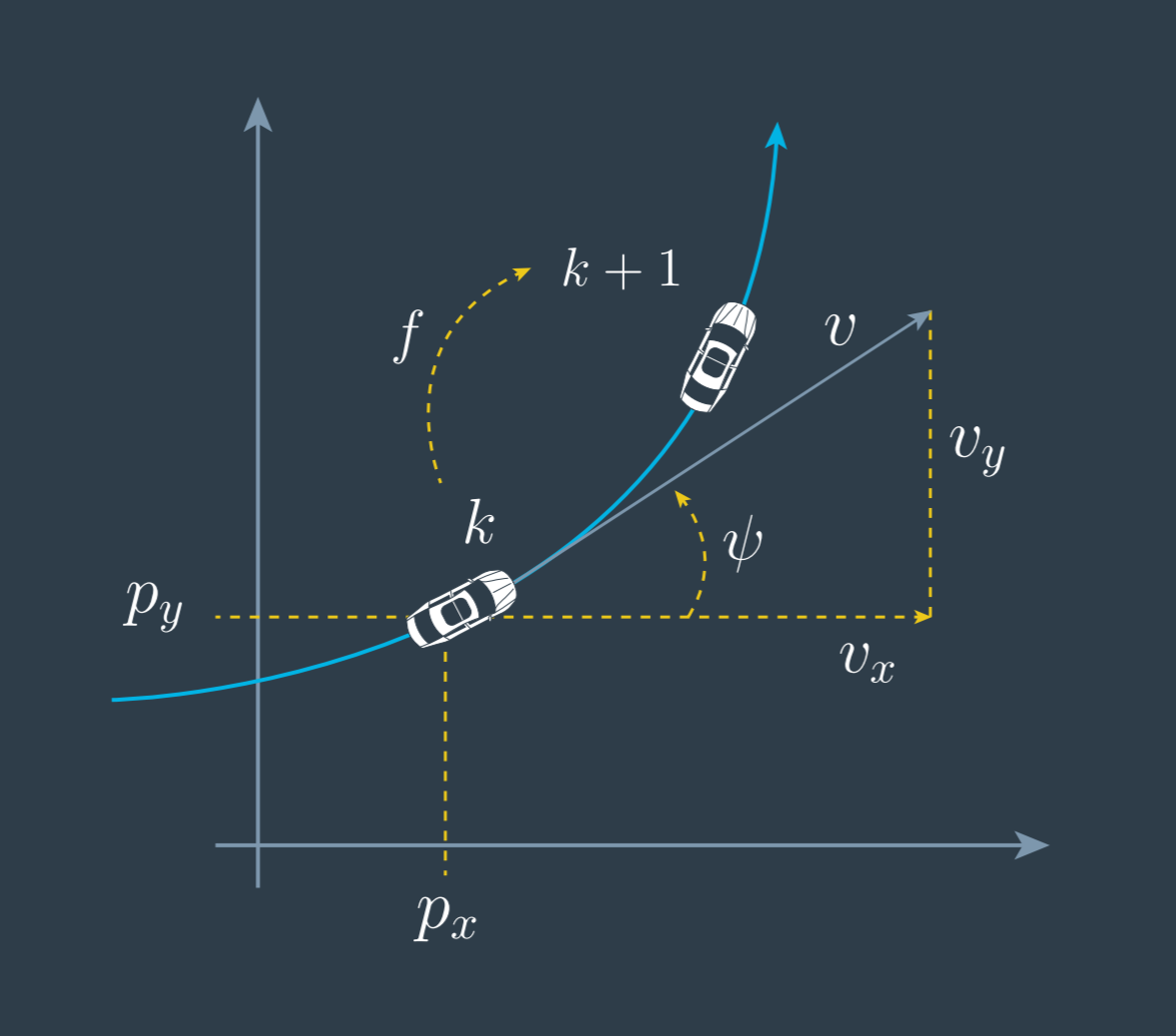
UKF 可采用匀速圆周运动模型,CTRV(Constant Turning Rate and Velocity model)
状态方程或过程模型(Process Model)
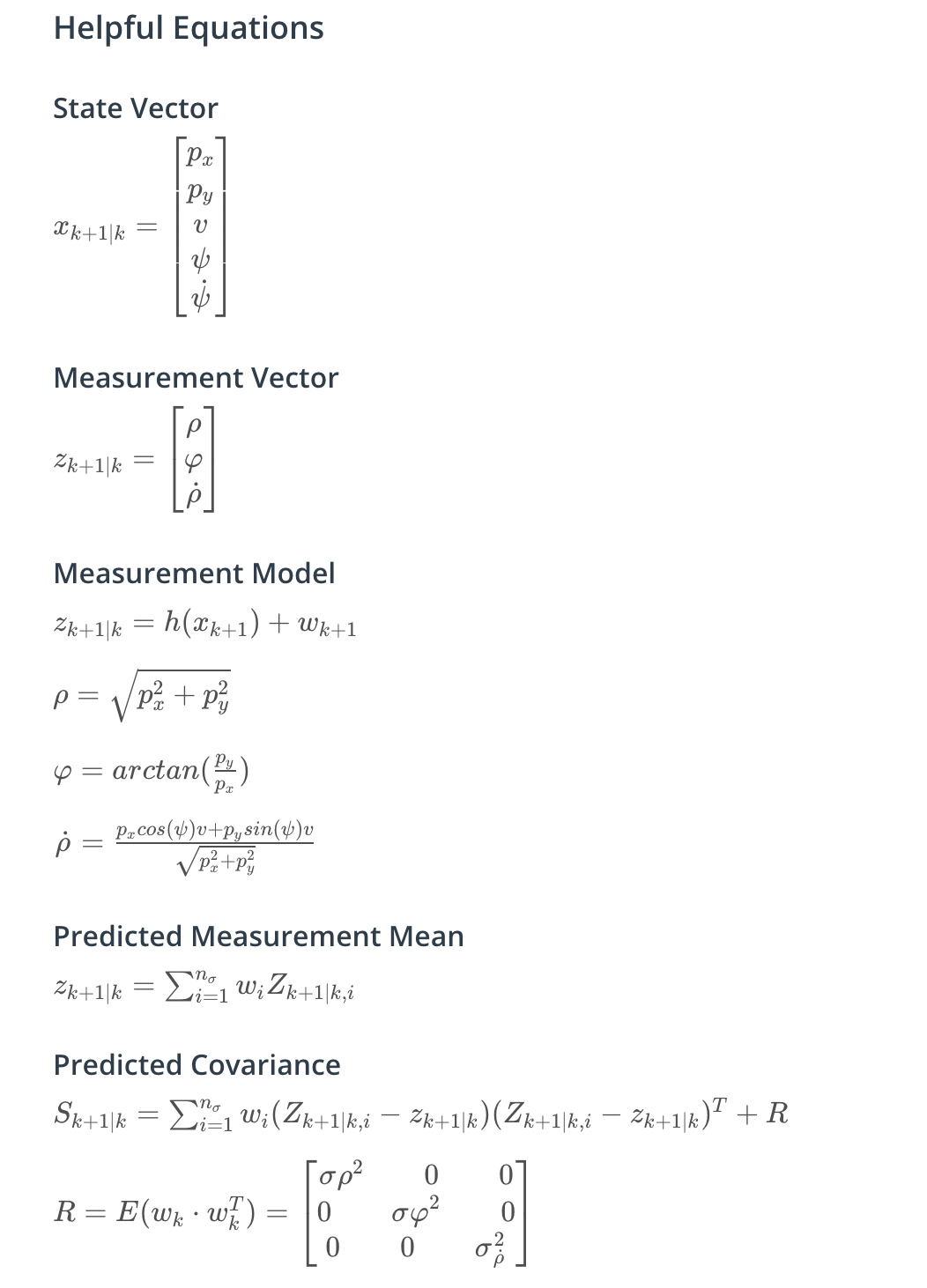
状态向量(state vector)选取
$$ x = (p_x, p_y, v, \psi, \dot {\psi}) $$
状态方程或过程模型(process model)如何得到,一个比较通用(general)的方法就是求解状态在两帧之间的变化量(Change Rate of State),其实就是状态量关于时间的微分。
$$
\dot x = (\dot p_x, \dot p_y, \dot v, \dot \psi, \ddot {\psi})
$$
$$
=(v\cdot cos\psi, v\cdot sin\psi, 0, \dot \psi, 0)
$$
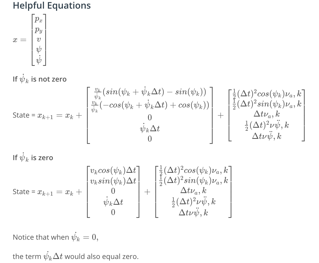
Process Model: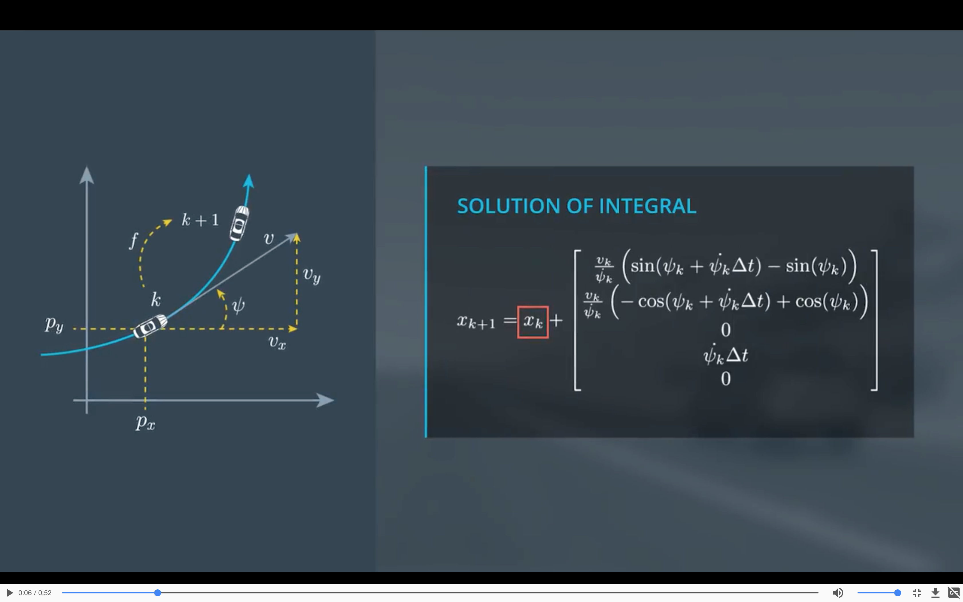
当yaw rate是0的时候,也就是直线运动时,因为状态转移方程中,前两项含有$\frac{v}{\dot \psi}$上述方程会发生奇异,所以当yaw rate为0时,转移矩阵要略作修改为:
$$
x_{k+1} = x_k + (v_k\cdot cos\psi_k\cdot \Delta t, v_k\cdot sin\psi_k \cdot \Delta t, 0, 0, 0)^T
$$
上述是过程模型确定部分(deterministic part),还要再加上随机部分(stochastic part),由于纵向加速度和角速度会因为各种情况随机地发生,根据中心极限定理,叠加的加速度会成高斯分布,所以可以将这两部分加速度处理成噪声加入到过程模型中。
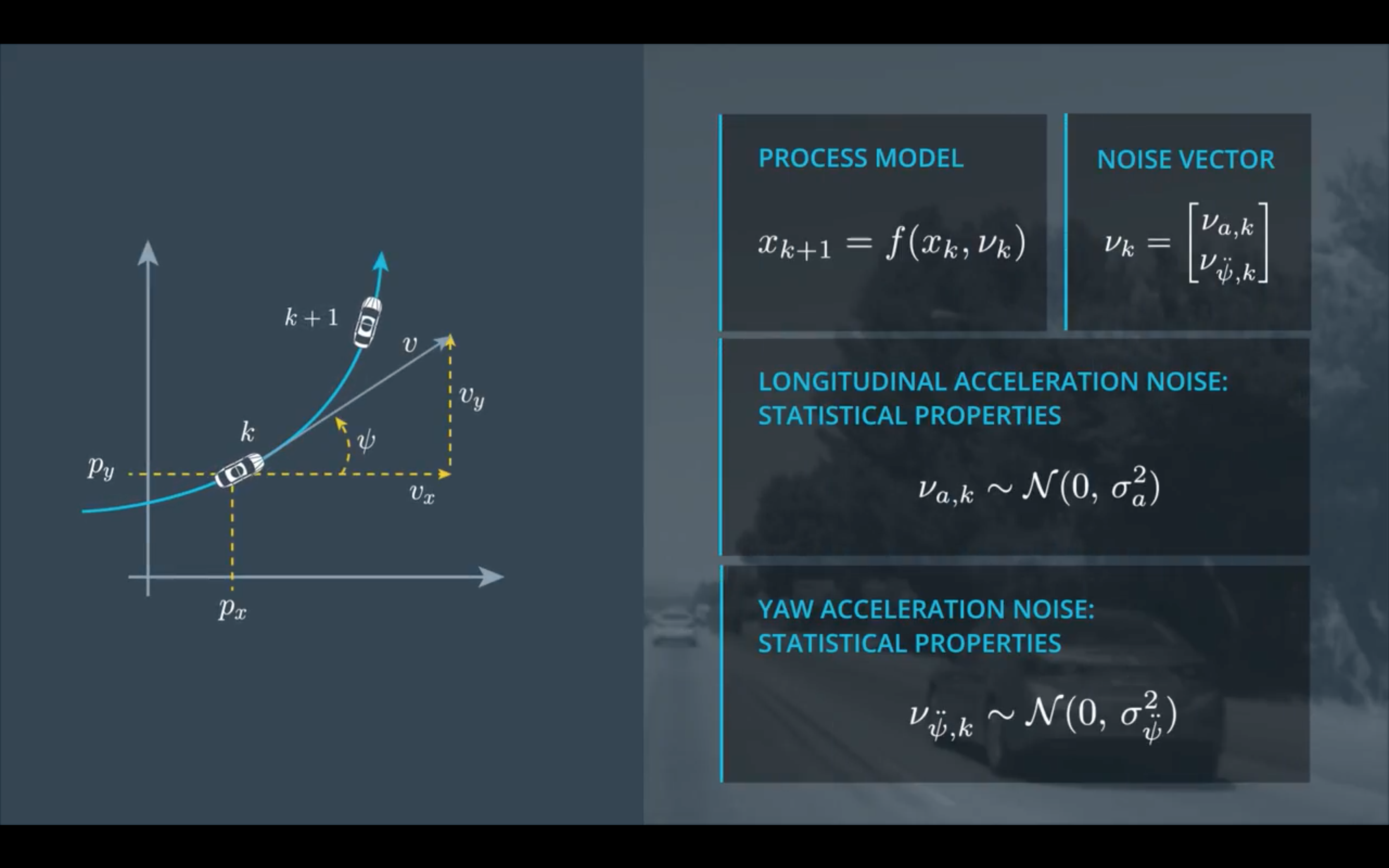
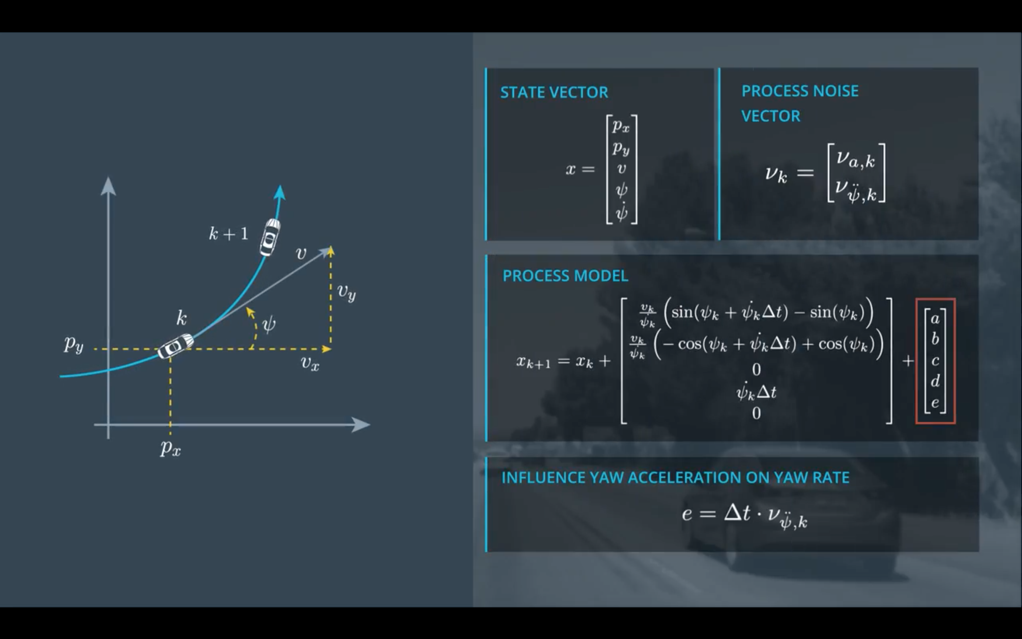
假设在连续两帧之间,线加速度和角加速度都为常数,并且位置噪声噪声做一阶近似,那么可以得到上述
$$
a = 1/2\nu_{a,k} \cdot cos\psi_k \cdot \Delta t^2
$$
$$
b = 1/2\nu_{a,k} \cdot sin\psi_k \cdot \Delta t^2
$$
$$
c = \nu_{a,k} \cdot \Delta t
$$
$$
d = 1/2\nu_{\ddot \psi,k} \cdot \Delta t^2
$$
$$
e = \nu_{\ddot \psi, k} \cdot \Delta t
$$
Pipeline
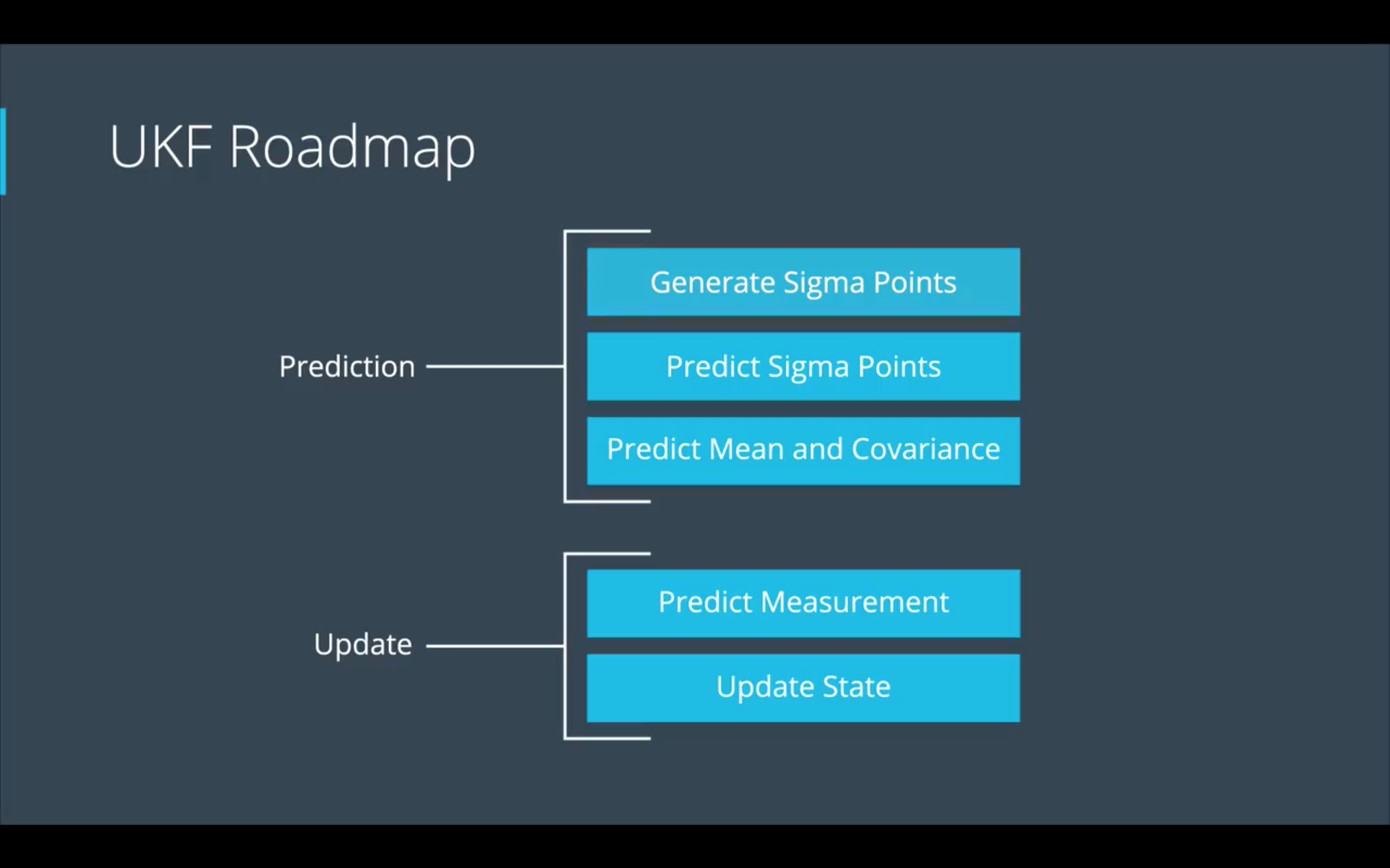
预测(Prediction)
生成Sigma 点
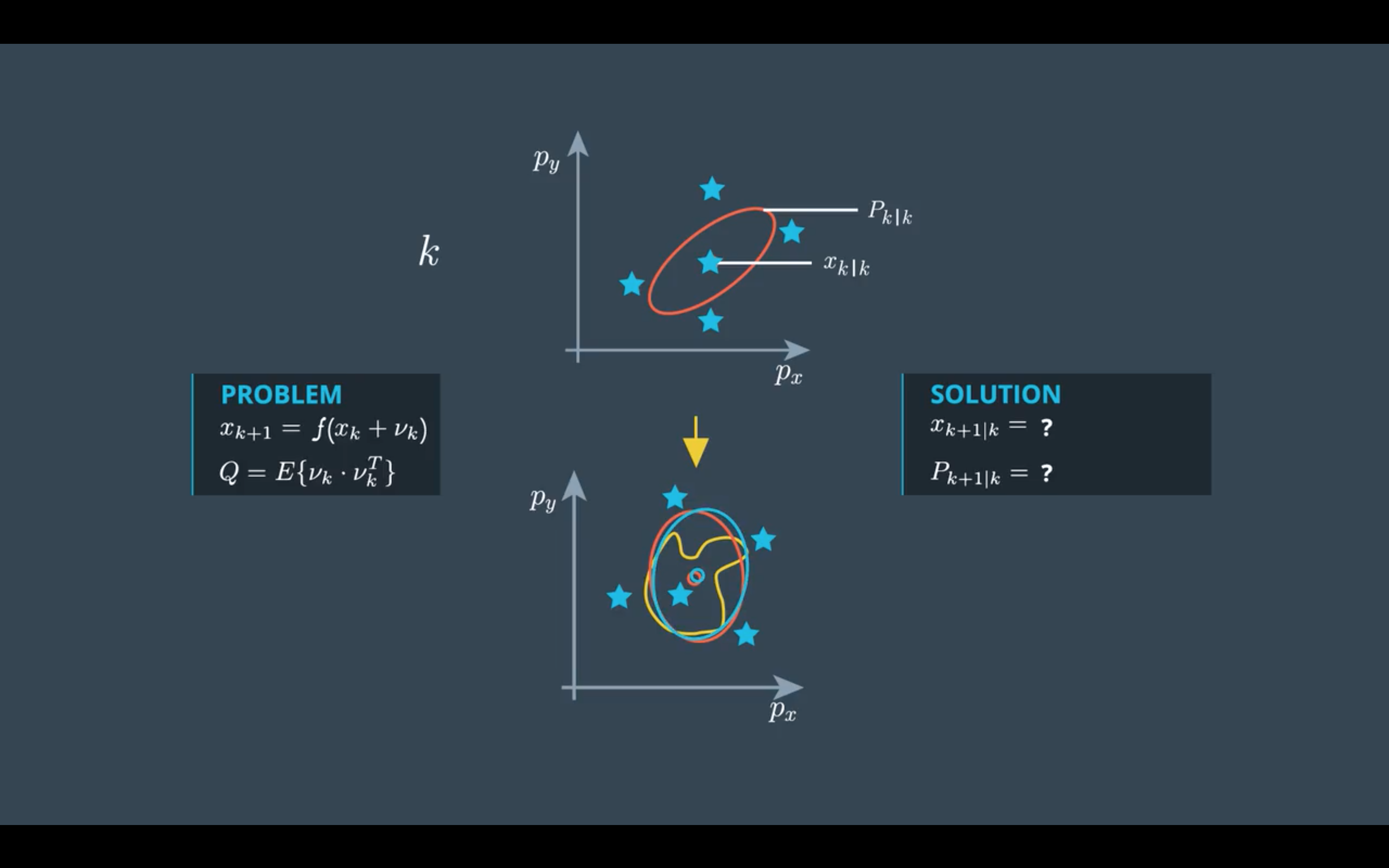
UKF也是为解决非线性模型诞生的(这个非线性有可能是状态转换的非线性也有可能是测量的非线性),但不同于EKF求解Jacob矩阵或是Hessian矩阵将非线性函数线性化(相当于将整个分布通过线性化的转移函数映射到了预测空间);相反,UKF选择的是将原状态空间里的某些具有代表性的点(这个代表性指的是这些点能代表整个分布的特点),即所谓Sigma点,通过非线性转移函数映射到预测空间,在预测空间中再去计算这个Sigma点的均值方差,用另一个高斯分布来近似数据在预测空间的分布。
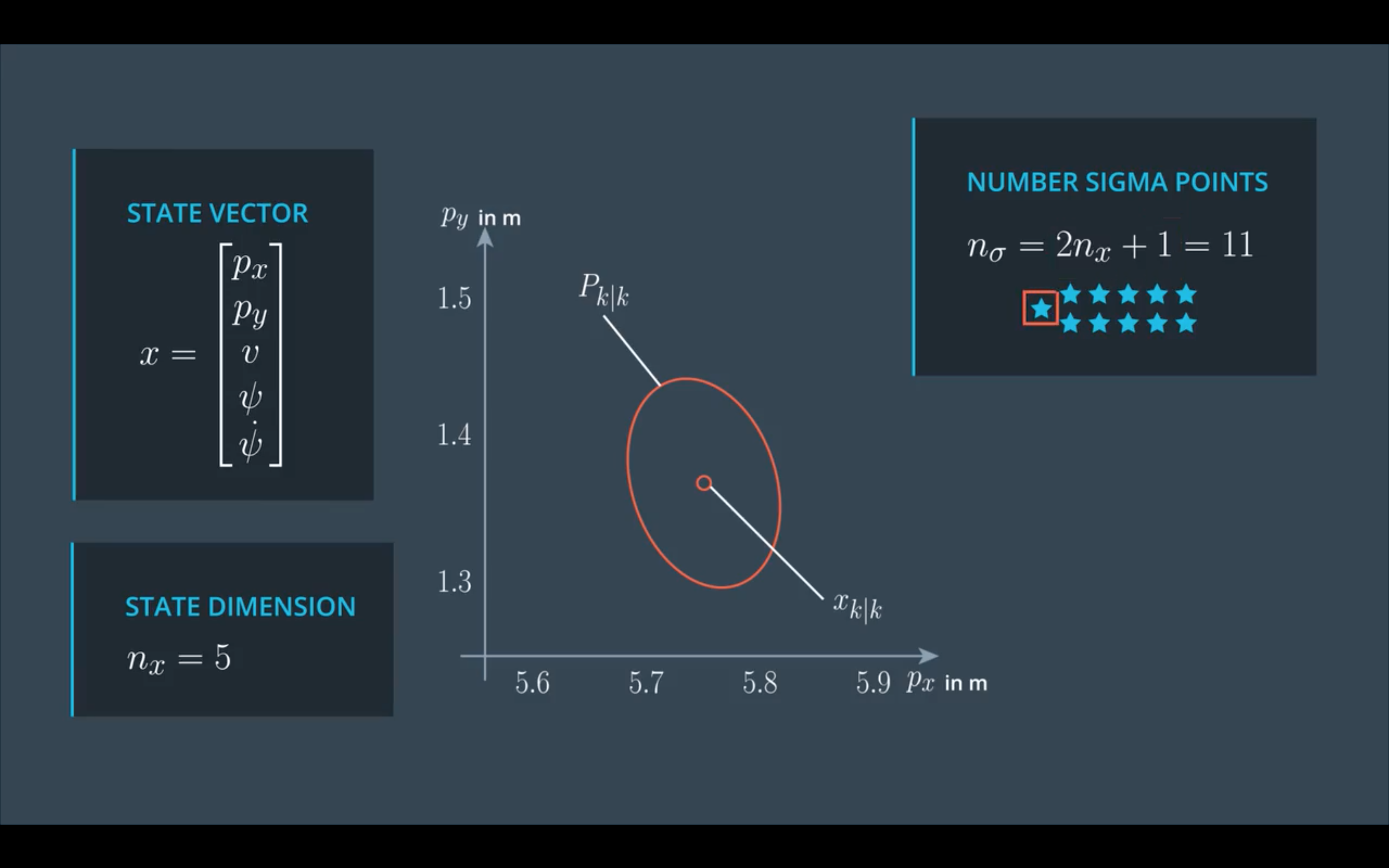
Sigma点数量与当前状态向量维度($n_x$)有关:
$$
n_\sigma = 2n_x + 1
$$
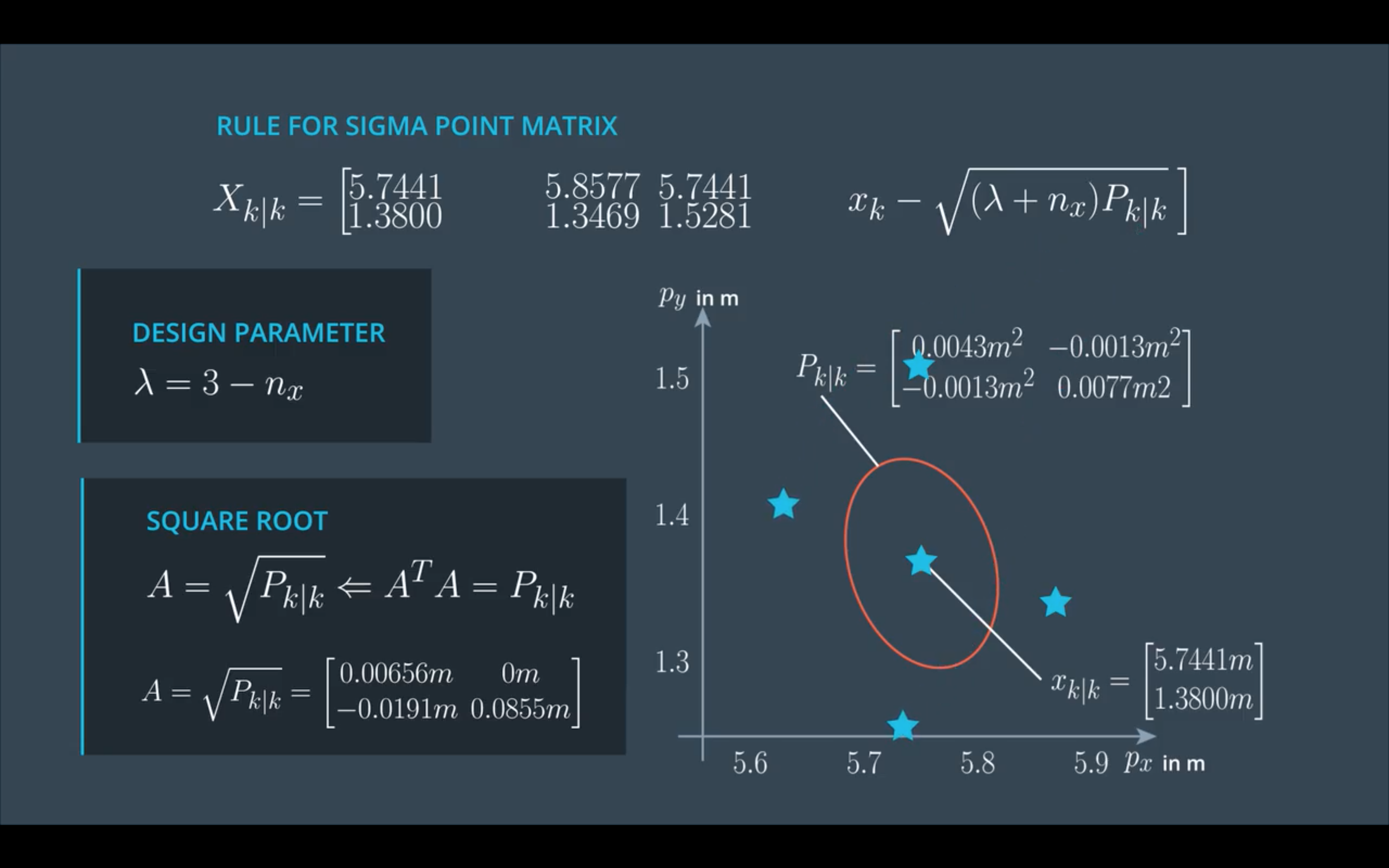
sigma 点计算公式:
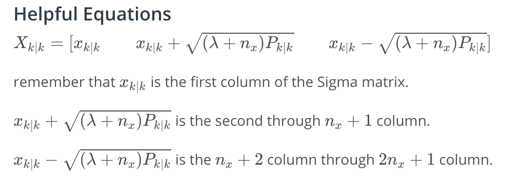
第一个sigma点就是均值点,$\sqrt {P_{k|k}}$是$n_x$个sigma点的方向,$\lambda$可以用来设置这些sigma点距离均值点的远近。
下面这张图假设状态量只有位置(x,y):
代码, GenerateSigmaPoints():
|
|
预测sigma点
接下来需要将sigma点通过非线性方程(如下)映射到预测空间的sigma点。
但是在这个过程中需要用到噪声$\nua$和$\nu{\ddot \psi}$。在UKF中对噪声的非线性处理非常简单,将其也加入到sigma点生成中,得到增广sigma点矩阵。
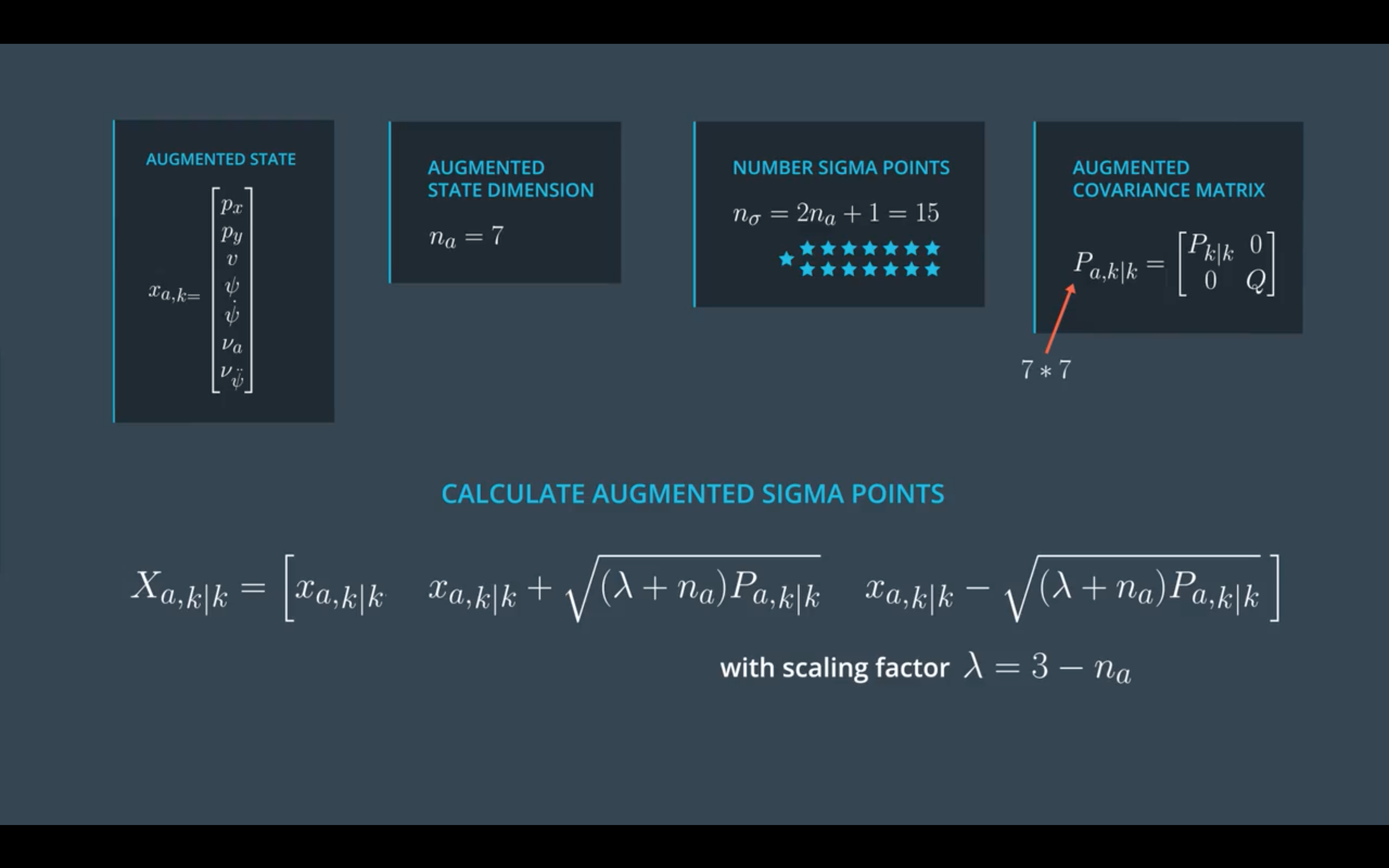
这样子便可以将增广sigma矩阵中的每个sigma点代入到非线性过程函数$f(x_k, \nu_k)$中得到预测的状态量。
代码,AugmentedSigmaPoints()和SigmaPointPrediction() :
|
|
|
|
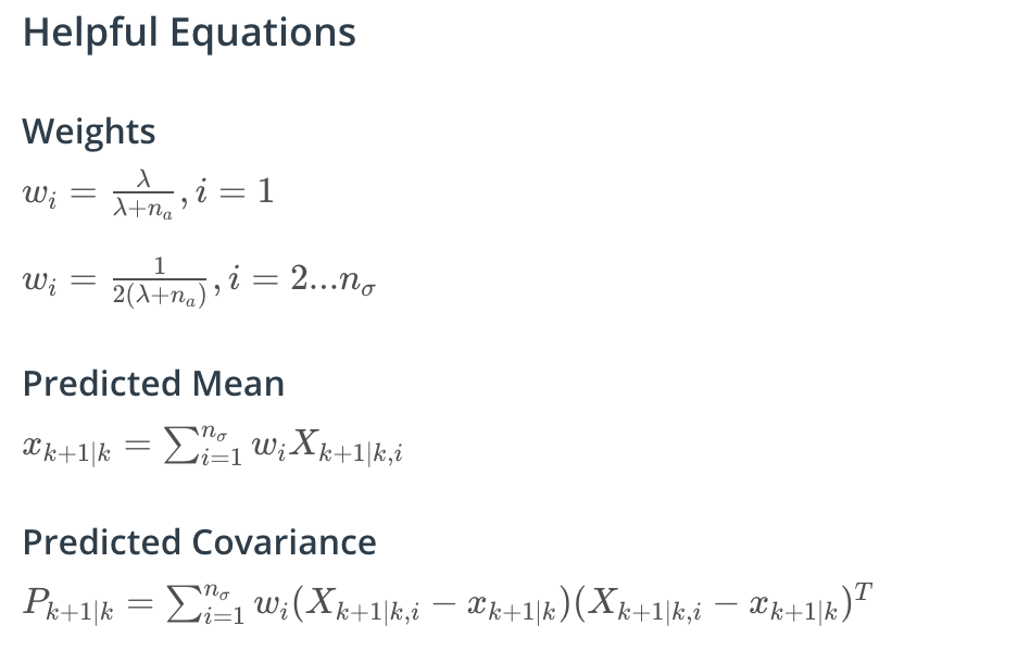
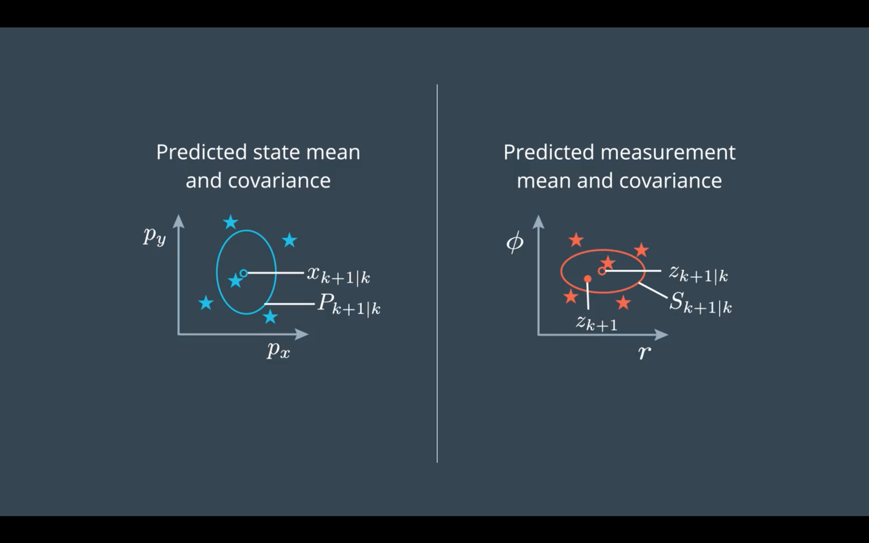
预测均值和方差
在预测空间计算新sigma点的均值和方差,均值是这些点的加权平均,方差也是加权方差,系数如下:
代码,PredictMeanAndCovariance() :
|
|
更新(Update)
预测观测值( Predict Measurement)
KF更新阶段需要将状态向量映射到观测空间,计算与观测量点残差进行状态更新。在UKF中,这一步的操作同样用sigma点来进行替代,将sigma点映射到观测空间的方法与预测阶段的相同,并且过程可以更简单。
- sigma点不需要重新生成,重复利用预测空间的sigma点(这些sigma点是从状态空间映射过来的)即可。
- 因为观测噪声是直接加在观测量上的(即观测噪声本来就在观测空间,映射关系中不会用到),所以映射过程不涉及观测噪声,也就无需计算增广sigma点矩阵。
.png)
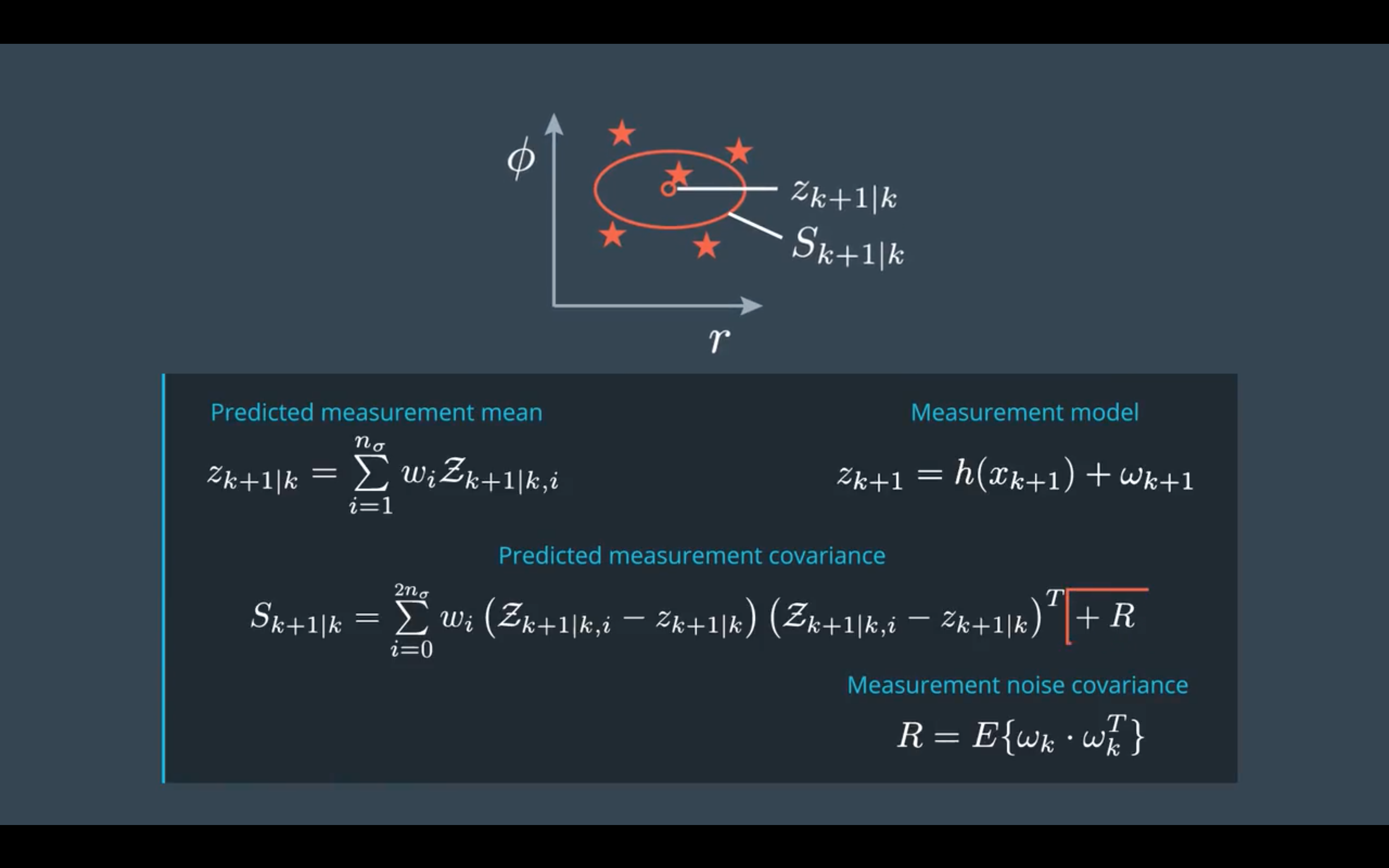
假设使用Radar数据作为观测量,
代码,PredictMeanAndCovariance() :
|
|
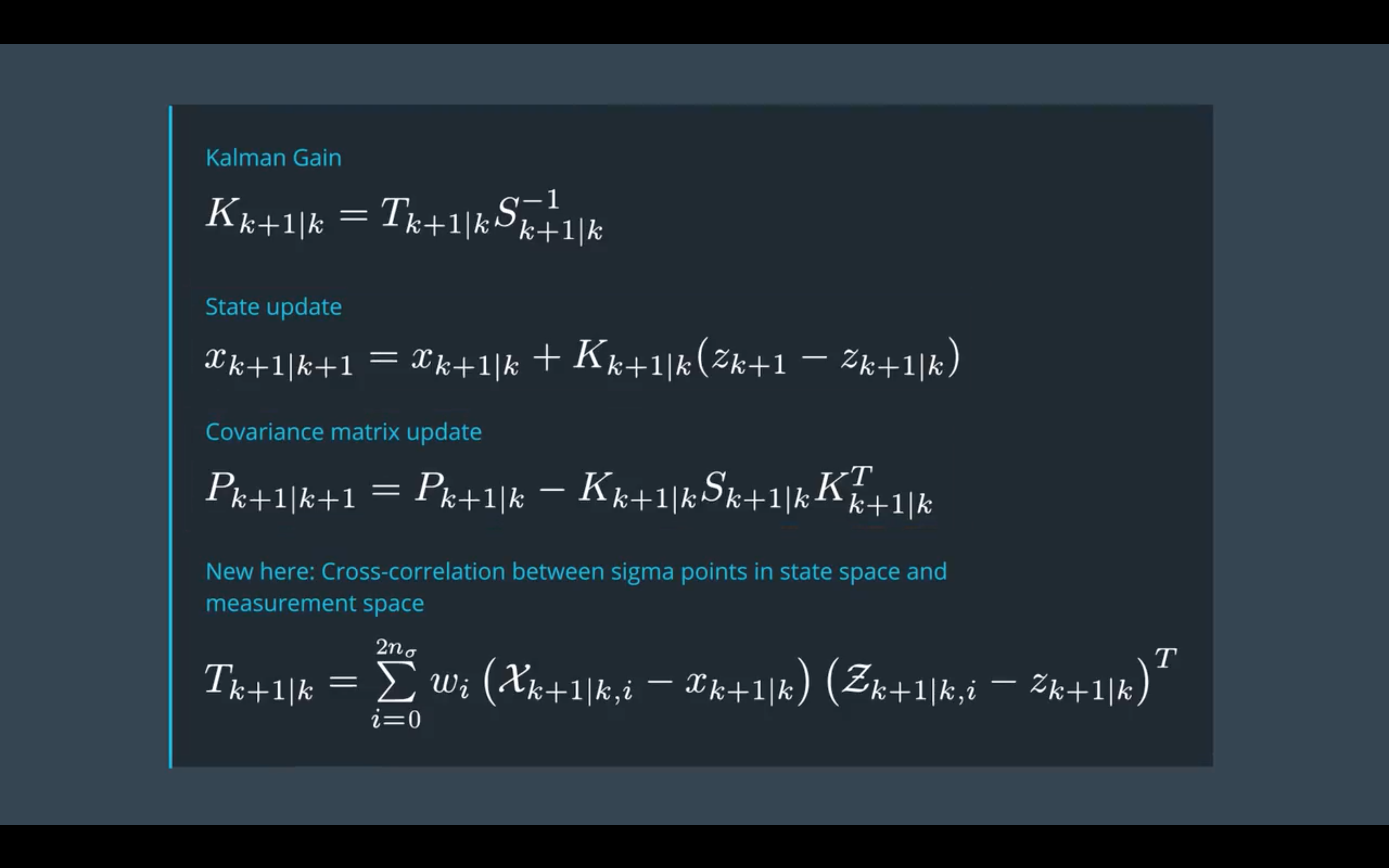
状态更新(State Update)
现在我们需要利用观测值进行状态更新了(是的,之前的步骤中都没有涉及到观测值)。
code,UpdateState():
|
|
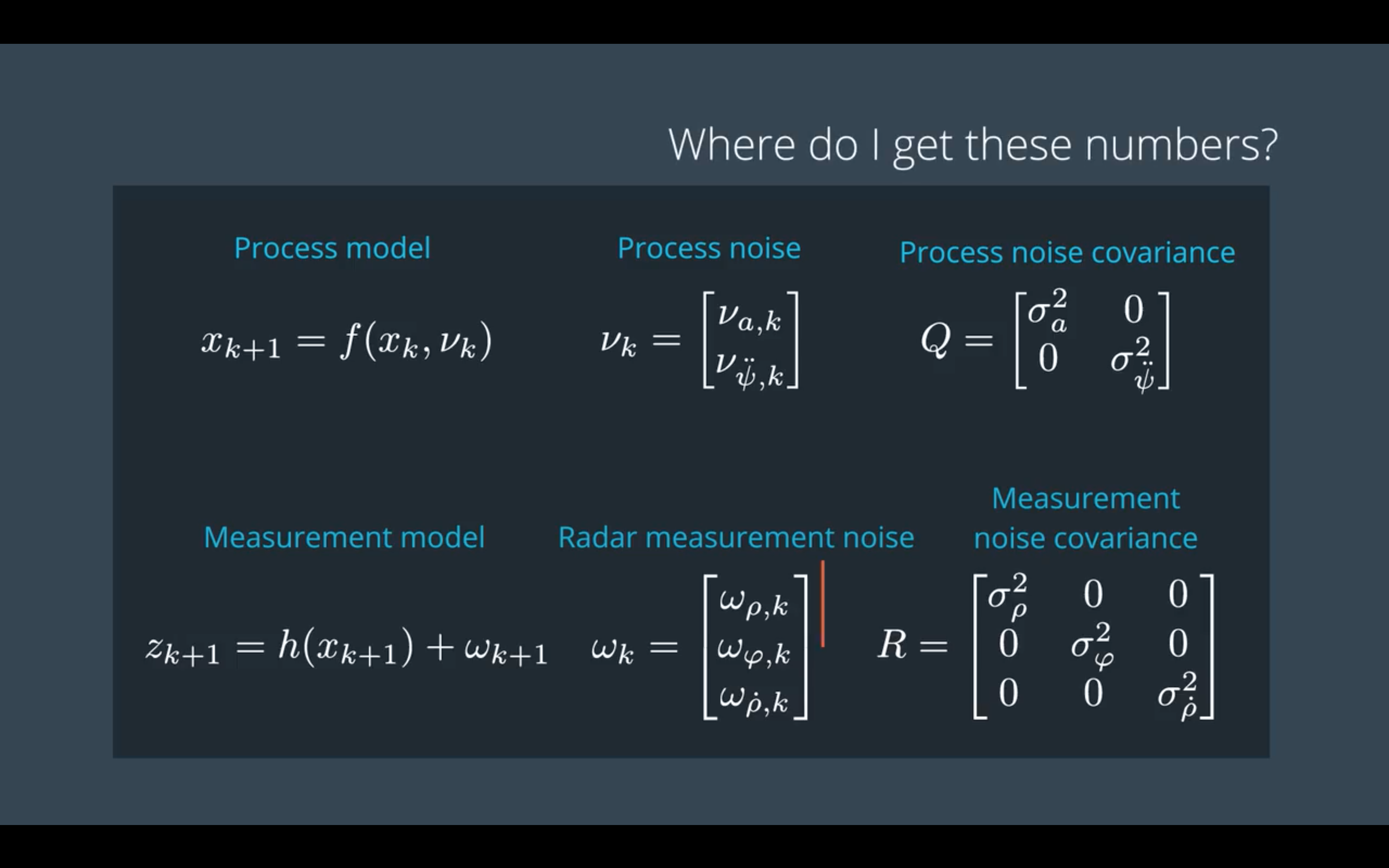
参数与一致性(Parameter and Consistency)
不管是KF,EKF还是UKF我们都需要设定噪声参数,噪声都认为是标准高斯分布的,所以只需要设定噪声的标准差即可。
测量噪声(Measurement Noise)
测量噪声一般需要查看传感器说明书,一般会有提供。若没有,可以通过静态试验的方法得到统计量,然后根据自己的实际需要测试,微调测量噪声。
过程噪声(Process Noise)
过程噪声只能根据物理意义来进行估计了。高斯分布95%的点落在$2\sigma$内,标准差量纲和噪声一致,所以这对估计很有用。
比如纵向加速度噪声$\nu_a$,一般汽车的加速度都在$6m/s^2$以内,所以取$\sigma_a = 6/2 = 3$,就比较合理了;如果追踪目标是自行车或是行人,那么$\sigma$值又要相应降低。
再比如角加速度$\nu_{\ddot {\psi}}$,用高中物理知识我们知道圆周运动角加速度和切向加速度关系是$a_r = \frac{a_t}{R}$,跟转弯半径关系很大。假设线加速度最大只能$6m/s^2$,转弯半径在10m左右,那么角加速度也只能是$0.6 s^{-2}$,那么加速度噪声
$$
\sigma_{\ddot {\psi}} = 0.6/2 =0.3
$$
是较为合理的。
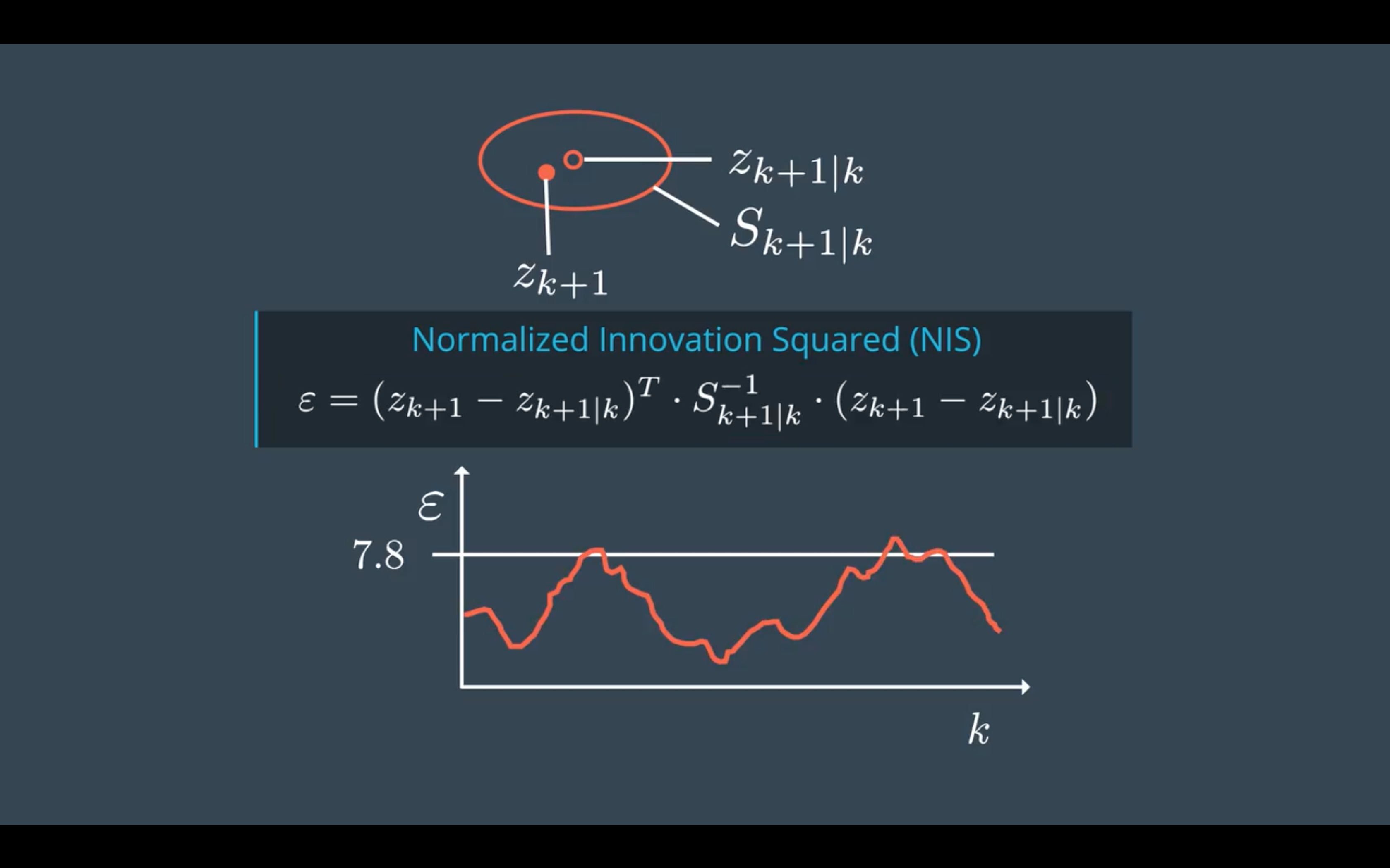
一致性评估(Consistency)
噪声的参数选择是否合适,可以用正则化的平方新息NIS(Normalized Innovation Squared)进行评估。
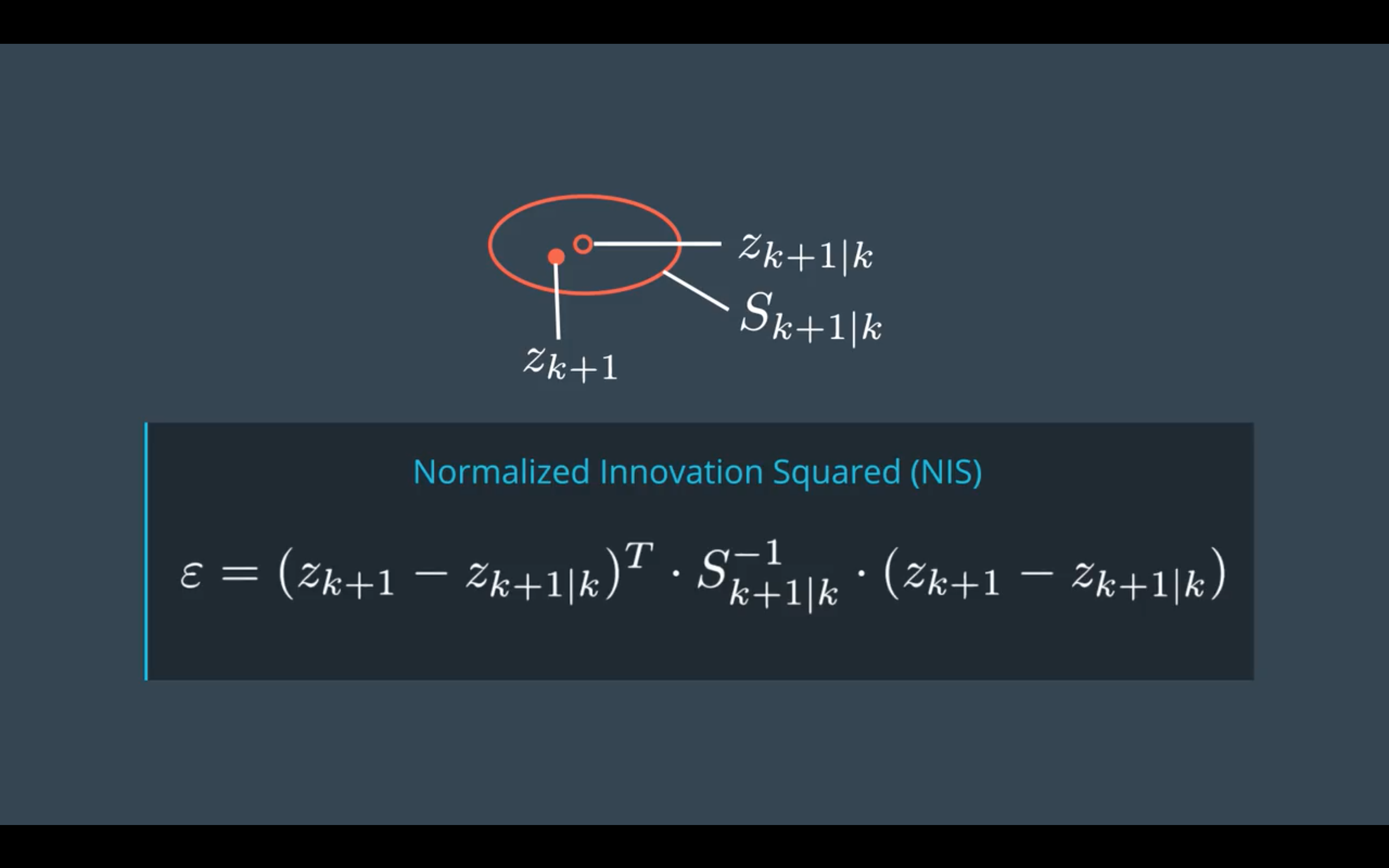
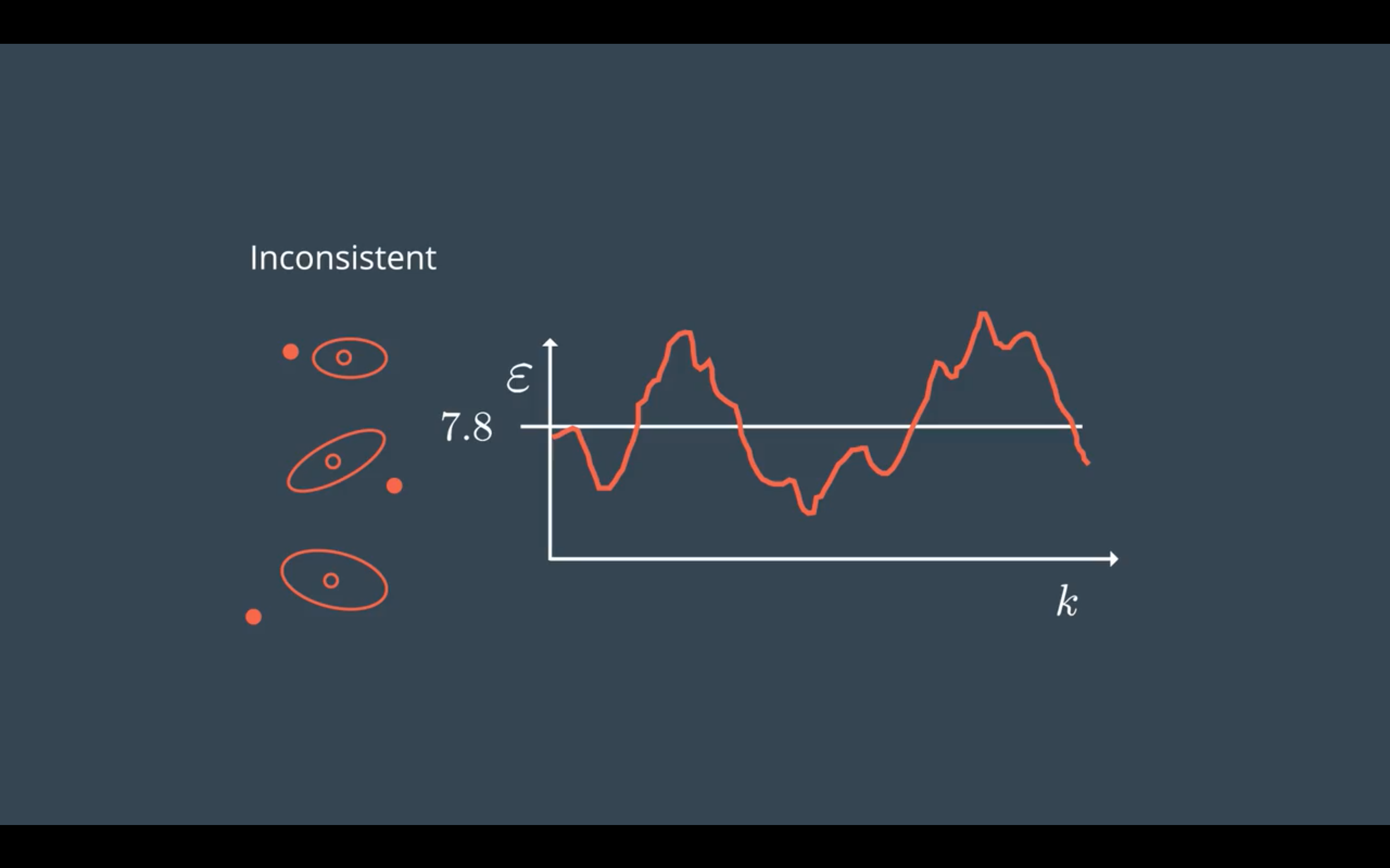
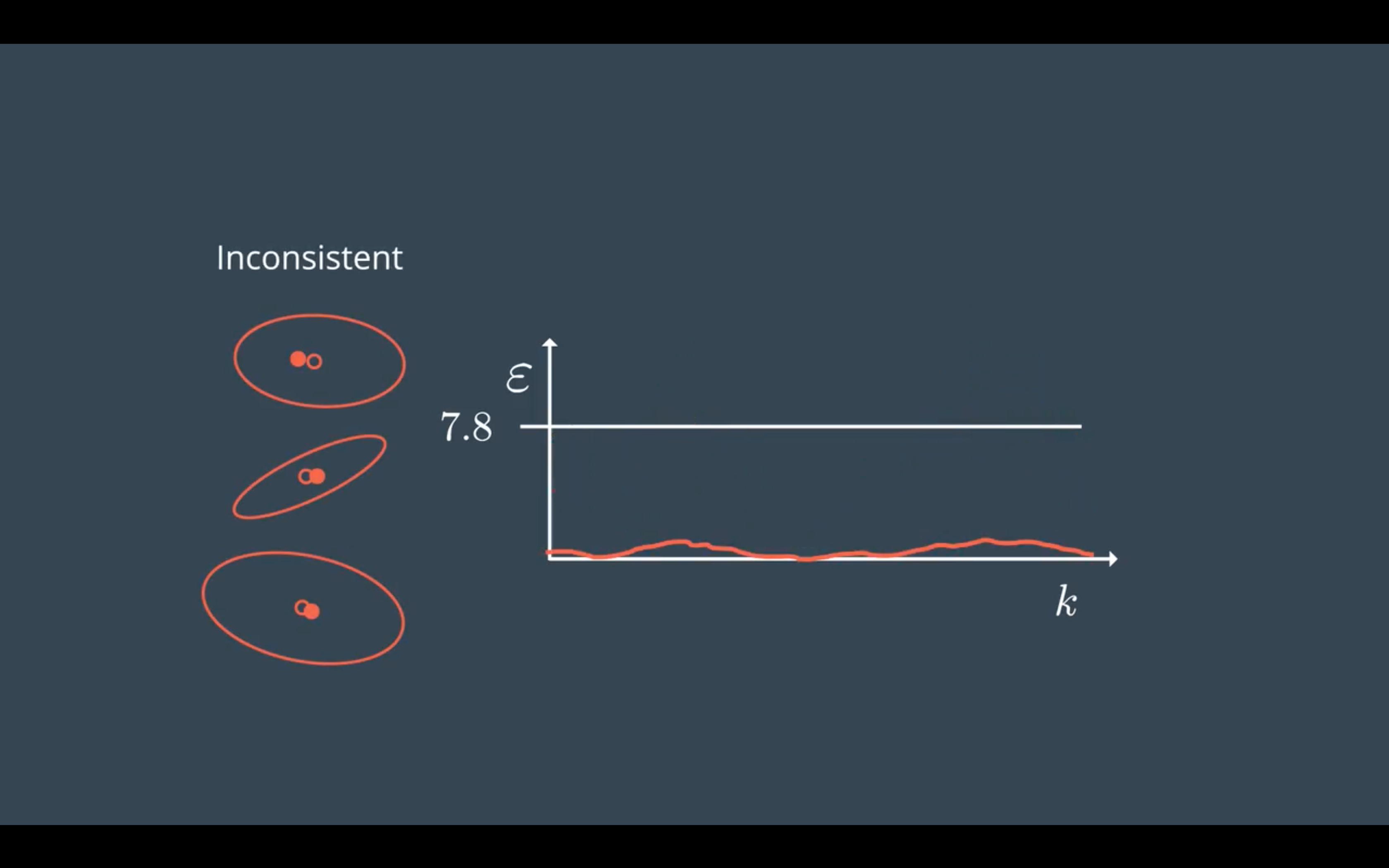
NIS满足卡方分布,下面三种情况分别是 满足一致性要求,低估不确定性(underestimate uncertainty),高估不确定性(overestimate uncertainty)